Purpose
A plot is a great way to summarise statistics and the
groveR package ships with functions to create two, one for
a vegetation density class and the other for extent change.
Use the ...plot() functions
The plots created are stacked barcharts. They also use some of the area calculations that have already been run. Each function will output one plot per unique region/site combination found in the csv file.
The veg_dens_class_plot() function uses the csv output
from running the veg_class_area() function which is found
in the extent_summaries/ directory.
# The general form of the function is (NOTE there are no default parameters)
# veg_dens_class_plot(icsv, areaname, cap)

# We  need to assign all of the parameters
icsv <- "extent_summaries/lgcsmp_lsat_2007-2023_extent_summaries.csv"
areaname <- "lgcsmp_lsat"
cap <- "produced by RSSA"

# Run the function
veg_dens_class_plot(icsv, areaname, cap)
icsv - input csv. It will only work with the extent summaries csv as output from the
veg_class_area()function.areaname - a geographical area or marine park name for the plot output.
cap - whatever is input here appears as a caption below the plot. If nothing is required use ““.
The extent_change_plot() function uses the csv output
from running the extent_change() function which is found in
the extent_change/ directory.
# The general form of the function is (NOTE there are no default parameters)
# extent_change_plot(icsv, areaname, cap)

# We  need to assign all of the parameters
icsv <- "extent_change/lgcsmp_lsat_2007-2023_extent_change.csv"
areaname <- "lgcsmp_lsat"
cap <- "produced by RSSA"

# Run the function
extent_change_plot(icsv, areaname, cap)
icsv - input csv. It will only work with the extent change csv as output from the
extent_change()function.areaname - a geographical area or marine park name for the plot output.
cap - whatever is input here appears as a caption below the plot. If nothing is required use ““.
What’s going to happen?
Running veg_dens_class_plot() will create a plot like
this:
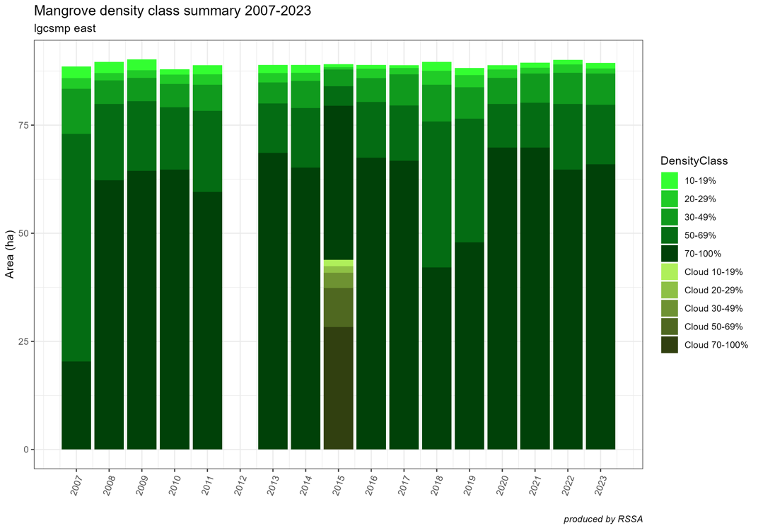
Note that there was no data for 2012.
Running extent_change_plot() will create a plot like
this:
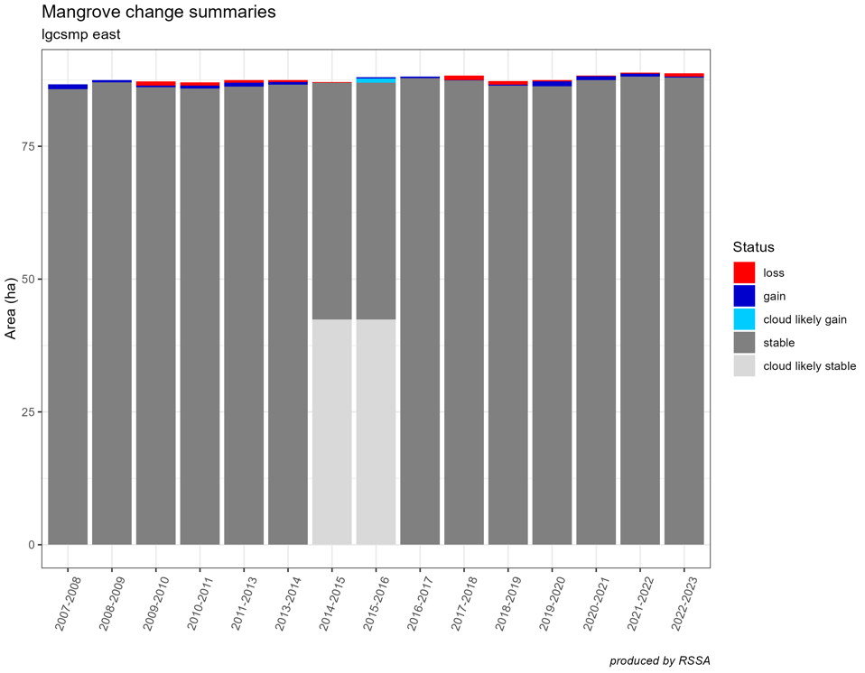
Note that with 2012 data missing from the time series, the chart displays change in extent between data for 2011 and 2013.
NOTE on plotting. Plots can be made in a variety of styles, focus on certain data ranges only or be formatted in a multitude of ways. It is beyond the scope of this package to attempt to provide code to anticipate all of these options. The data in the csv’s is however in an easily manipulated format. For ideas on how to manipulate the data to construct alternate plots please examine the code for these two functions in the GitHub repository.
If you have been following along the vignettes in order, this one is
the last describing a typical workflow using the groveR
package. Happy processing!