Purpose
This stage is similar to calculating the vegetation class areas however this time we are calculating the trend class areas.
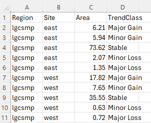
Use the trend_class_area() function
The trend_class_area() function takes the trend class
bins and reports on their respective areas. In order to report
effectively, a region needs to be delineated. This boundary needs to be
supplied in a shapefile. Convention has it that an attribute column,
named “region” contains a region name and a site name separated by an
underscore. An example might be “lgscmp_east”, “lgscmp_west” etc. This
should be the same shapefile that was used when running the
veg_class_area().
# The general form of the function is (NOTE there are no default parameters)
# trend_class_area(irast, iregions, attribname)

# We  need to assign all three of the parameters
irast <- "trend_class/lgcsmp_lsat_2014-2023_trendclass.tif"
iregions <- "vectors/regions.shp"
attribname <- "regions"

# Run the function
trend_class_area(irast, iregions, attribname)
irast - file path to the trend class raster for a distinct period that has been written to the
trend_class\directory. If multiple periods (and rasters) exist, run the function for them one at a time.iregions - file path to a shapefile denoting the reporting region.
attribname - the name of the attribute column containing region information.