Install and load the package
You only need to install the package once (unless you are updating
it). The package lives on GitHub so you will need devtools
to install.
# Install and load groveR
# install.packages("devtools")
devtools::install_github("dbca-wa/groveR")
library(groveR)
Once this is done you need to set up a standard processing environment.
Why?
The functions in this package are going to require access to various data and will produce raster and csv products. If everything is located in a standard structure your analysis will run smoother and you won’t be inclined to lose anything.
How?
It is strongly recommended that you use an RStudio project. Either create one from scratch or create one from an existing directory. This will now become your working directory and all file paths are relative to this. If you do not wish to use RStudio then the same effect can be achieved by setting your working directory to a folder that makes sense to you.
The next stage is to use groveR to setup a directory
tree. These folders will be used to house various data and many of
groveR's functions will default to looking in them for
required data.
# Make the sub-directories in the processing folder
make_folders(p =".")
What does it look like?
The sub-directories have the following structure:
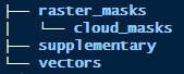
These directories will contain user supplied data:
raster_masks/will contain “general” raster masks of the type that will be applied to all satellite data.raster_masks/cloud_masks/will contain “specific” raster masks that will be applied only to certain satellite data dates.supplementary/will contain three csv files. One each to describe calibration coefficients, density classes and trend classes.vectors/will contain a shapefile that delineates the region that output area stats are generated for.
What’s next?
The starting point for this workflow is a directory containing pre-generated annual vegetation index rasters that cover an area to be reported on. These index rasters, one per year, will have been chosen on the basis of:
- An appropriate index, when used in a model, provide the best measure of cover.
- That the time of capture is the same for all time steps i.e. the same season.
- That at the time of capture it was low tide as water underneath mangrove canopies confounds the analysis.
- That they are free from cloud. Where cloud is unavoidable, the cloud
has either been digitised and a corresponding shapefile has been stored
in
vectors/, or a cloud mask has been created and stored inraster_masks/cloud_masks/. - That they cover the whole area of interest. If the area of interest is larger than an available satellite scene, multiple scenes have been mosiacked together to produce the index raster.
- That the source data for the index rasters all come from the one satellite source, i.e. all Landsat or all Sentinel.
- That they all have identical extents (footprints) and pixel sizes.
The above mentioned index data will be large and as such may not be located in the Processing Folder. You will however need to know where it is and be able to provide a file path to it’s location.
The other data that you will need to provide will be stored in the appropriate sub-directories of the described Processing Folder. Ensure any masks have the same extents and pixel sizes as the annual rasters. The required csv files will be described in detail later in the vignettes as will any shapefile.
A Note on Projections
Any data that is used for your analysis must have a consistent projection. As reporting areas used in mangrove monitoring can straddle more than one UTM zone, Albers Australia (EPSG: 3577) has been used as a default. This is a reasonable choice as it enables easy calculation for area in metres and UTM zones are not an issue. All outputs will be in EPSG:3577 and functions will check and re-project inputs if they differ.