Purpose
The next step is to calculate the area of each vegetation class per year. The tabulated results can then be used to create plots.
Use the veg_class_area() function
The veg_class_area() function takes the reclass bins and
reports on their respective areas. In order to report effectively, a
region needs to be delineated. This boundary needs to be supplied in a
shapefile. Convention has it that an attribute column, named “region”
contains a region name and a site name separated by an underscore. An
example might be “lgscmp_east”, “lgscmp_west” etc.
# The general form of the function is (NOTE the default parameters)
# veg_class_area(irast, iregions, attribname, areaname, ext = ".tif", probabilities = TRUE)

# We  need to assign four of the parameters as the other defaults are fine
irast <- "veg_class"
iregions <- "vectors/regions.shp"
attribname <- "regions"
areaname <- "lgcsmp_lsat"

# Run the function
veg_class_area(irast, iregions, attribname, areaname)
irast - input vegetation classification directory.
iregions - file path to a shapefile denoting the reporting region.
attribname - the name of the attribute column containing region information.
areaname - a geographical area or marine park name for the output csv.
What’s going to happen?
A csv of areas in hectares will be output to the
extent_summaries\ directory and will look similar to
this.
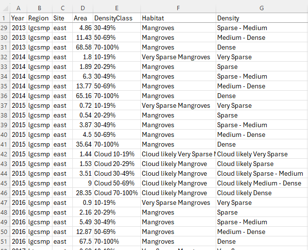
The above shows the example data for 2013-2016 and also demonstrates
what happens if there was cloud in one of the mosaics (2015) and the
default parameters were used. The probabilities = TRUE
parameter tells the function that if a pixel is cloudy then report on
what it might have been considering what the pixel was the year before.
If you change the default to probabilities = FALSE then
just the area of cloud is reported on.