Purpose
The vegetation density rasters, whilst useful, presently contain continuous values which are a little unwieldy when analysing and summarising. The next step in the processing workflow is to “bin” the continuous values into meaningful groupings.
Use the veg_class() function
We now apply the veg_class() function to our masked veg
density outputs. If there has never been cloud in any of the mosaics
then you can use the veg_dens_mskd\ directory (lucky you),
however the veg_dens_mskd_cld\ directory is the
alternative. The function will apply the user determined density classes
found at supplementary/density_classes.csv. The example
shipped with the package most likely contains the correct values but as
always, if unsure please check. Below is a screenshot of shipped data,
make sure you follow the same format if changes are required.
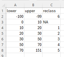
The above example shows the lower and upper limits to bin the continuous values into the reclass value. Here, densities of between 0-10 are ignored and values above this fall into 5 density bins (1-5). The reclass value of 6 is reserved for cloud (cloud masking encoded the affected pixels to -99 in a prior step).
# The general form of the function is (NOTE the default parameters)
# veg_class(irast, ext = ".tif", classes = "supplementary/density_classes.csv")

# We only need to assign one of the parameters as the defaults are fine
irast <- "veg_dens_mskd_cld"

# Run the function
veg_class(irast)- irast - input vegetation density directory.
What’s going to happen?
The input vegetation density rasters will be reclassified according
to the density classes provided in the csv file and will be written to
veg_class/ directory. Whilst these raster layers can be
useful as visualisations, in this workflow they will be summarised by
area and this will be covered in the next vignette.