How to make plots and tables for annual reports

Introduction

All water quality data, historical and present, is accessed through the Water Information Reporting portal maintained by the Department of Water and Environment link. Data should be downloaded for the Canning Estuary and the Swan Estuary sites using the keywords search terms “SG-E-CANEST” and “SG-E-SWANEST” respectively. Data requested should be “Water Quality (discrete) for Site(s) cross-tabulated” and as the data size is large, requests should be split into appropriate yearly chunks. This data is the starting point for using the functions that follow to produce plots and tables for the annual reports. It is suggested that the original downloads be kept and the data simply updated yearly.

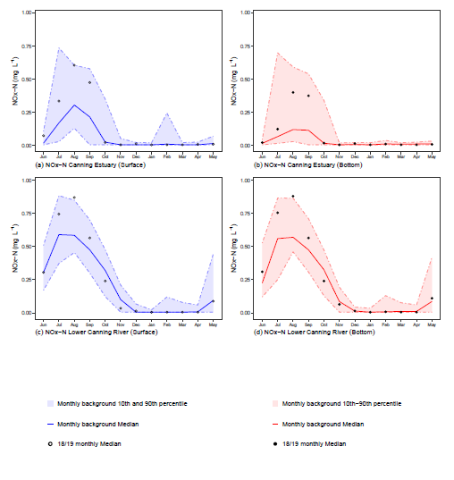
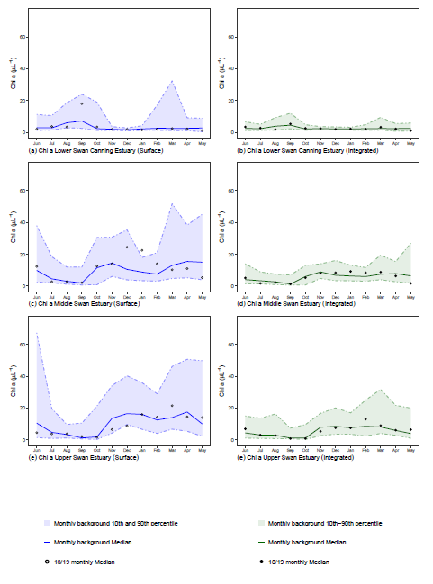
The plots created by the functions are output as panel plots and follow the same format as previous annual reports. A panel is based on a variable and contains a separate plot for each combination of ecological management zone (emz) and sampling method. Visualisation consists of:

a “ribbon” designating the 10th and 90th percentiles of the background data
a line showing the background data median
points showing the current reporting period medians

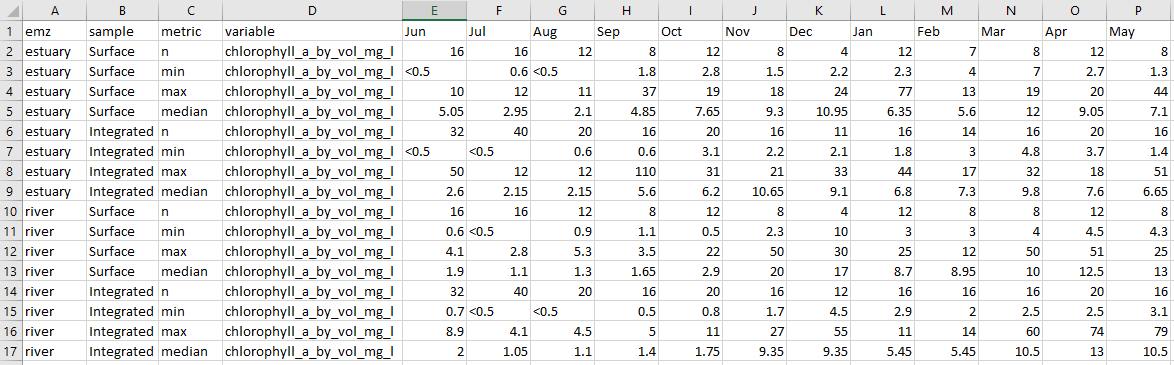
The tables generated from the same functions contain counts, minimums, maximums and medians for the current reporting period per month. These are summarised by emz and sampling method and can be copied straight into the report when it is being compiled.

The process for creating the plots and tables has two stages.

Stage One - Data assembly

Data required for the annual reports consists of a current reporting period (01 June to 31 May) and background period (5 years prior to current reporting period). In this stage all downloaded data is read in and categorised into a current and background period. The downloaded data has some challenging formatting (for automatic reading and variable naming etc) so these functions are very specific to the current export format. Should this format change these functions will fail and require some editing.

When the report is read in it is tidied with the following occuring:

variable names are standardised
values are checked for “<” or “>”:
- a value following a “<” is halved
- a value following a “>” is left as is
the variable emz is created based on site

Once the data is read in and tidied it is exported as a csv with the format “XX-X-XXXXX_annual_report_data_for_YYY.csv” where:

“XX-X-XXXXX” is the estuary (i.e. SG-E-CANEST or SG-E-SWANEST)
“YYYY” is the current reporting year.

Remember to change the file path slashes if on a Windows OS. Examples below.

#load the package
library(rivRmon)

#Canning estuary - forward slash example
canning_WIN_report_data(inpath = "C:blah/blah/annual_data_location", 
                        reportingYear = 2019, 
                        outpath = "C:blah/blah/somewhere")

#Swan estuary - backslash example
swan_WIN_report_data(inpath = "C:blah\\blah\\annual_data_location", 
                     reportingYear = 2019, 
                     outpath = "C:blah\\blah\\somewhere")

inpath is a character file path to the downloaded data xlsx files reportingYear is a 4 digit numerical representing current reporting year outpath is a character file path to desired export location for writing of the csv files

This function needs to be run each year to set up the data for the annual report. The output from this stage will be the input for the next two stages.

Stage Two - Creating plots and tables

There is a separate function for each estuary. These are essentially wrapper functions around other functions that work on data that has the same requirements for visualisation (mainly formatting such as plots per panel, or data filtering parameters etc). Outputs are saved to directories created by running the functions. There will be a panels and a tables directory with the prefix “c_” or “s_” for Canning and Swan estuaries respectively.

#Canning estuary - forward slash example
canning_reportR(inpath = "C:blah/blah/somewhere", 
                outpath = "C:blah/blah/somewhere_else", 
                surface = "blue", 
                bottom = "red",
                chloro = "darkgreen")

#Swan estuary - backslash example
swan_reportR(inpath = "C:blah\\blah\\somewhere", 
                outpath = "C:blah\\blah\\somewhere_else", 
                surface = "blue", 
                bottom = "red",
                chloro = "darkgreen")

inpath a character file path to pre-made annual report data (the out path from Stage 1 above)

outpath a character file path to desired export location

The parameters surface, bottom and chloro can take a named colour or a hex colour code. The defaults produce colours similar to those produced in prior reports, however access to these parameters allows users to tweak if required. surface relates to surface measurements, bottom to bottom measurements and chloro to integrated measurements specific only to chlorophyll plots.

Examples

Canning estuary total oxidised nitrogen.

Swan estuary chlorophyll a.

Chlorophyll a csv table

Groupings of variables

As stated previously some variables are grouped so that code can filter data under similar circumstances. These groupings are as follows.

For the Canning estuary:

chlorophyll a - by itself
dissolved organic carbon - by itself
group 1
- total nitrogen
- ammonia nitrogen
- total oxidised nitrogen
- dissolved organic nitrogen
- total phosphorus
- filterable reactive phosphorus
group 3
- dissolved oxygen
- pH
- salinity
- temperature
secchi depth - by itself
silica - by itself

For the Swan estuary:

chlorophyll a - by itself
group 1
- total nitrogen
- ammonia nitrogen
- total oxidised nitrogen
- dissolved organic nitrogen
- total phosphorus
- filterable reactive phosphorus
- silica
group 2
- alkalinity (not report variable for Canning estuary)
- dissolved organic carbon
- tss (not report variable for Canning estuary)
group 3
- dissolved oxygen
- pH
- salinity
- temperature
secchi depth

Note that swan_reportR outputs 2 panel plots as per the original report for the group 3 variables. The extra panel plots are for the additional emz of “Swan”.

Plotting individual variable groupings

As previously mentioned, the reportR functions are wrappers. The individual functions are available to the user and can be found in the reference index. The groupings match the above and function names take the format ann_rep_vvvv_e() where:

“vvvv” is the variable or grouping
“_e” is the estuary (“_c” or “_s”)

As these functions are written to be internal to the wrapper they need to be run in the following manner in order to read in the correct data.

#load additional packages
library(tidyverse)

#setup a file path to the annual report data (i.e. csv from Stage One)
inpath <- "C:path/to/anuual_report_data"

#get the full name and pathrow to the required data - change pattern as required
file <- list.files(path = inpath, pattern = "SG-E-CANEST_annual_report", 
                   full.names = TRUE)

#create parameter variables for the function you want to use
outpath <- "C:path/to/desired_export_location"
data <- readr::read_csv(file = file, guess_max = 10000)

#run function - here we have chosen group 1 variables for the Swan
ann_rep_grp1_s(outpath, data, surface = "blue", bottom = "red")