Getting started
one.Rmd
Welcome to the FireHistory package!
FireHistory is an R package designed to assist
researchers get the best out of the Department of Biodiversity,
Conservation and Attraction’s (DBCA) fire history dataset
(DBCA_Fire_History_DBCA_060). The fire history is a very large spatial
polygon dataset comprising of collated fire events (prescribed burns and
bushfires) that have occurred on departmental lands. Earliest records
date from 1937 and the data is updated regularly. The data can be
accessed on the data
WA website.
There are 3 main steps in the FireHistory workflow:
- Downloading data
- Getting the data prepped for analysis
- Generating metrics
Downloading the Fire History dataset
The FireHistory package relies on the DBCA dataset to be
downloaded and available locally. Unfortunately at this stage an API
workflow is not available. As the data is dynamic care must be taken to
ensure that the data downloaded is the latest available.
To download the data please follow this link data
WA website. Go to the Data Downloads drop down menu and
click the download for shapefile button. This button will take you to
the Shared Location Information Platform (SLIP) managed by Landgate. You
will need to register and login as a user. Access is free and the login
requirement is for statistics only. Once logged in you will have the
ability to download the data in two different Datums. Please choose the
GDA2020 version.
At time of writing the download was 939MB and should take a few minutes depending on connection speeds. Make sure you save it somewhere locally on your computer and remember how to get to it.
While on the data WA website, also click on the
Resources drop down menu and download the PDF of “Look-up
Tables”. This has important information about the attribute columns in
the downloaded shapefile if you wish to further understand and explore
the fire history data.
Data preparation
First things first, you will need to download the package and load
it. You can only install the package from the GitHub repository. If you
haven’t already installed R package devtools you will need
to do this first.
# install.packages("devtools")
devtools::install_github("dbca-wa/FireHistory")
library(FireHistory)
The basic workflow of data preparation is that a polygon/s representing an area of interest (AOI) will be used to spatially subset the DBCA fire history which will be further temporally filtered based on some user parameters. There are two options for defining an aoi.
User supplied AOI
Got your own shapefile that you would like to use? No problems.
# file path to your shape file - note includes the file extension
my_shape <- "C:/somewhere/myshapefile.shp"

# import it
aoi <- user_aoi(aoi_path = my_shape, name = "A very meaningful name")
Make sure your shapefile has a coordinate reference system. There
doesn’t need to be any specific information in the attribute table and
there can be multiple polygons if necessary as long as when assessed
together it makes sense. The parameter name should be
something helpful as all your products and plots will feature this.
DBCA tenure or forest block AOI
Want to use a National Park boundary or a forest block as the AOI but don’t know how to get it or what it’s full name is? No problems. The package ships with a complete listing of tenure and forest block names as well as their boundaries.
# For DBCA tenure - have a look at the first few records....there's 1000+
head(find_tenure())
#> [1] "Highbury Nature Reserve"
#> [2] "Badgingarra National Park"
#> [3] "Dwellingup State Forest"
#> [4] "Karnet Nature Reserve"
#> [5] "Myalup State Forest"
#> [6] "Recherche Archipelago Nature Reserve"

# Or for DBCA forest blocks
head(find_block())
#> [1] "CORNWALL"  "STOATE"    "GERVASSE"  "CATTERICK" "JASPER"    "TALLING"
That could take a while. Say we are pretty sure our National park AOI has something to do with wandoo.
# search for something like wandoo
find_tenure(like = "wandoo")
#> [1] "Wandoo National Park"    "Wandoora Nature Reserve"

# there are a few close matches but we want the first one and save it to an object
location <- find_tenure(like = "wandoo")[1]
Alternatively, we might be looking for a forest block called Jasper
# search for something like jasper
find_block(like = "jasper")
#> [1] "JASPER"

# there is only one so no need to subset this time
location <- find_block(like = "jasper")
Now that we have the correct name we can retrieve the DBCA spatial
boundary and save it as our AOI. The DBCA_aoi function’s
default behaviour is to return a tenure boundary. For a forest block
make sure you add the extra parameter.
# if the aoi is a tenure location
aoi <- DBCA_aoi(choice = location)

# if the aoi is a forest block
aoi <- DBCA_aoi(choice = location, block = TRUE)
Whichever way you define an AOI these functions will return a list containing a spatial object and its name.
After defining the AOI, you use it to subset the downloaded fire history data.
# file path to the fire history data - note includes the file extension
path <- "C:/somewhere/DBCA_Fire_History_DBCA_060.shp"
# here we want to temporally restrict it to the period 1988-2022
wandoo_data <- assemble_data(fire_path = path, FYfrom = 1988, FYto = 2022,
                             aoi = aoi, accessed_on = "01/01/2023")

# works the same for a forest block
jasper_data <- assemble_data(fire_path = path, FYfrom = 1988, FYto = 2022,
                             aoi = aoi, accessed_on = "01/01/2023")
A couple of things to note here.Firstly the FYfrom and
FYto parameters. The years are financial years (July-June)
not calendar years (January to December). This is because, in the south
west, the fire season occurs predominantly during the summer months.
Bear this in mind if your aoi is in the north.
Secondly, the accessed_on parameter is for the user to
record the date of when they accessed the DBCA_Fire_History_DBCA_060
shapefile. This date stamp will appear as a caption on plots etc.
Whilst the fire history data is huge, as it is subset using the AOI prior to reading into memory, this process is reasonably fast (about 10-20 seconds for the wandoo data set). Saving it to an object (here called wandoo_data) is important as this will be passed along to the fire metrics functions. If there is nothing in the fire history for the AOI the function will return an error. The fire history is most complete on DBCA tenure and forest blocks and generally even better in more populous regions/areas.
Fire Metrics
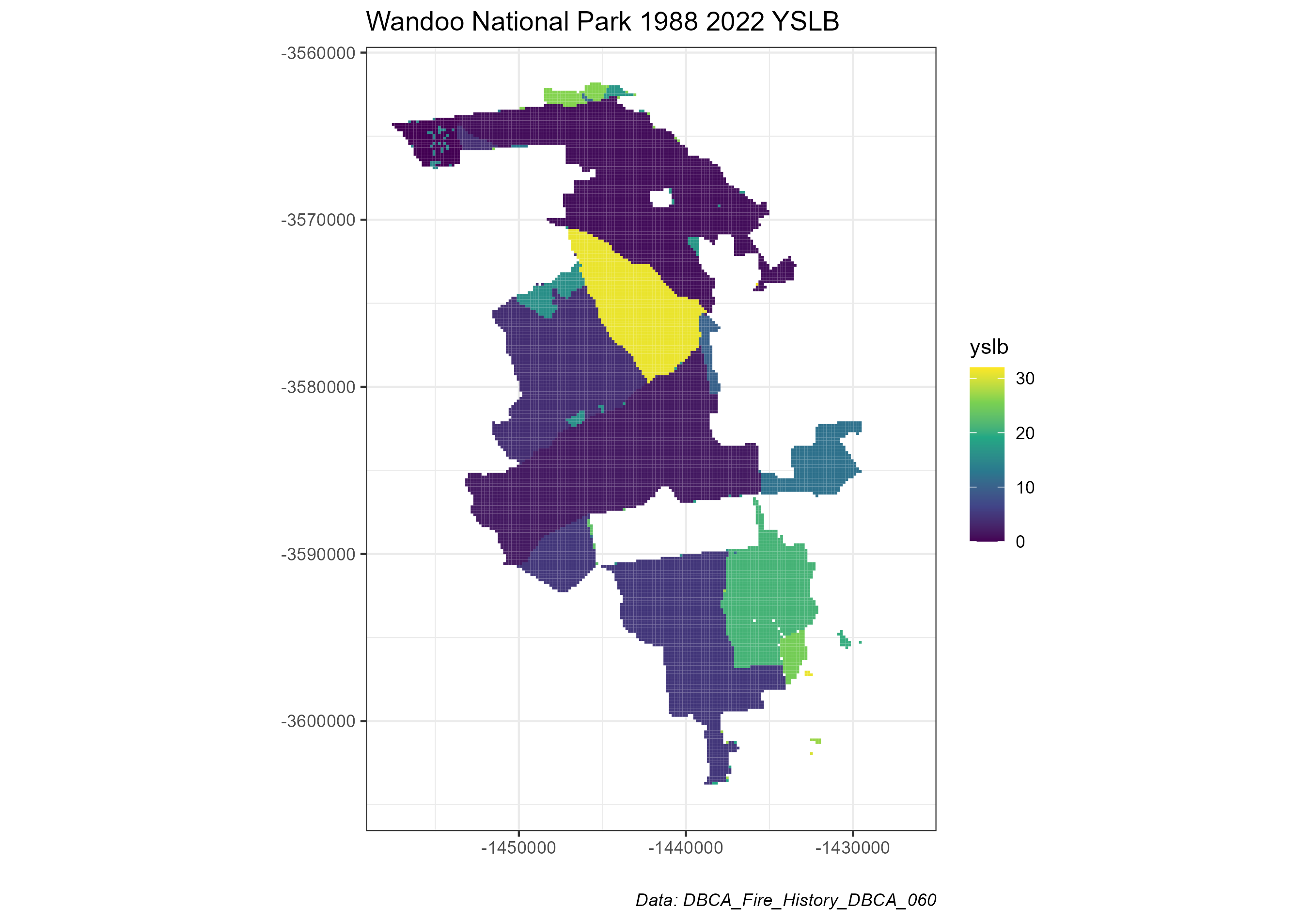
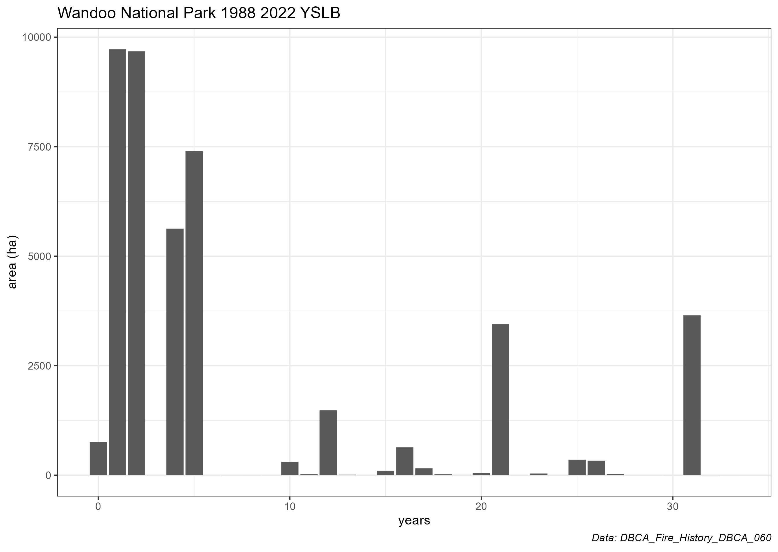
Now it is time to generate some fire metrics. Here is an example to calculate Year Since Last Burn (YSLB) for the Wandoo example above.
# create YSLB for the Wandoo National Park
yslb_list <- yslb(data = wandoo_data, products = TRUE)
By saving it to an object it creates a list containing:
- A YSLB raster of class SpatRaster (from the Terra R package)
- A YSLB map of class ggplot
- A tibble of area stats
- A YSLB column plot of class ggplot
By having a list of these products the user can extract them and
manipulate the plot objects or directly use the raster in other
analysis. The parameter products = TRUE will create a
folder in your working directory and save the four products to it.
Examples of the plots are below. 
