Data analysis - Producing insight from WAStD

Data

Load data

Download all the data live. This will take a while, but then allow to produce several reports (e.g. for different turtle programs) at once, or serve as data for an RShiny app like the turtle data preview.

data_wastd <- download_wastd_turtledata()

For a quick example, rendering this vignette, or skipping WAStD authentication, use the packaged data.

data("wastd_data")

Filter data

To filter records to one area, we can either filter by area or site ID , or simply filter by a bounding box. Additionally, we’ll filter by date.

Site names and IDs are only correct at the time of writing. As they could change, please double-check the correct spelling of your own place names and their IDs in WAStD’s Areas of type “Locality”.

seasons <- wastd_data$tracks %>%
  dplyr::group_by(season) %>%
  dplyr::tally() %>%
  dplyr::arrange(-n) %>%
  magrittr::extract2("season")

tracks <- wastd_data$tracks %>% filter_wastd_season(seasons[[1]])

Turtle Tracks and Nests

This section demonstrates the summary and visualisation utilities for tracks.

Maps

Each track on the map has a pop-up with a link to the actual record on WAStD. Accessing and editing the record is restricted to authorised DBCA staff members.

Map markers can be grouped or not.

Non-grouped markers show the actual location more accurately, but can overlap to the point where it is not possible to open the pop-ups. Maps with many markers can be slow to render.

Grouped markers in densely populated locations will expand to prevent the overlap of markers and pop-ups. Maps with many clustered markers render fast.

Use “Place names” where the aerial imagery is not available at the zoom level required for the grouped markers to expand.

wastd_data$tracks %>%
  map_tracks(sites = wastd_data$sites)

# Many tracks display more performant when clustered wastd_data$tracks %>% map_tracks(sites = wastd_data$sites, cluster = T)

Nesting success - tracks with nest vs the rest

Overview tables are available for the most common summaries at the most common groupings (season, week, day / area, site).

We show print-optimised knitr tables here, but could also use the more refined reactable (filterable, sortable, searchable) for interactive use.

wastd_data$tracks %>%
  nesting_type_by_season_species() %>%
  rt()

wastd_data$tracks %>% nesting_type_by_area_season_species() %>% rt()

wastd_data$tracks %>% nesting_type_by_site_season_species() %>% rt()

wastd_data$tracks %>% nesting_type_by_season_week_species() %>% rt()

wastd_data$tracks %>% nesting_type_by_season_day_species() %>% rt()

# Track success by day and species wastd_data$tracks %>% track_success() %>% rt()

# Track success by species wastd_data$tracks %>% track_success() %>% track_success_by_species() %>% rt()

wastd_data$tracks %>% track_success() %>% ggplot_track_success_by_date( "natator-depressus", placename = "Test place", prefix = "TEST" )

wastd_data$tracks %>%
  track_success() %>%
  ggplot_track_successrate_by_date(
    "natator-depressus",
    placename = "Test place", prefix = "TEST"
  )

Nest excavations: Hatching and emergence success

wastd_data$nest_excavations %>%
  hatching_emergence_success() %>%
  rt()

wastd_data$nest_excavations %>% hatching_emergence_success_area() %>% rt()

wastd_data$nest_excavations %>% hatching_emergence_success_site() %>% rt()

Tagged nests

wastd_data$nest_tags %>% map_nests()

Disturbed nests

wastd_data$tracks %>%
  dplyr::filter(disturbance == "present") %>%
  add_nest_labels() %>%
  map_tracks(sites = wastd_data$sites)

wastd_data$tracks %>% dplyr::filter(disturbance == "present") %>% add_nest_labels() %>% map_tracks(sites = wastd_data$sites, cluster = T)

Disturbances and predation

wastd_data$nest_dist %>%
  disturbance_by_season() %>%
  rt()

wastd_data$nest_dist %>% map_dist()

wastd_data$nest_dist %>% map_dist(cluster = T)

Animals

Live sightings: rescues, in water, tagging

wastd_data$animals %>%
  filter_alive() %>%
  map_mwi(sites = wastd_data$sites)

Dead sightings: strandings, mortalities

wastd_data$animals %>%
  filter_dead() %>%
  map_mwi(sites = wastd_data$sites)

Surveys

All plots can be exported as a PNG file with export = TRUE.

pl <- "Western Australia"
pr <- "WA"

wastd_data$surveys %>%
  surveys_per_site_name_and_date() %>%
  rt()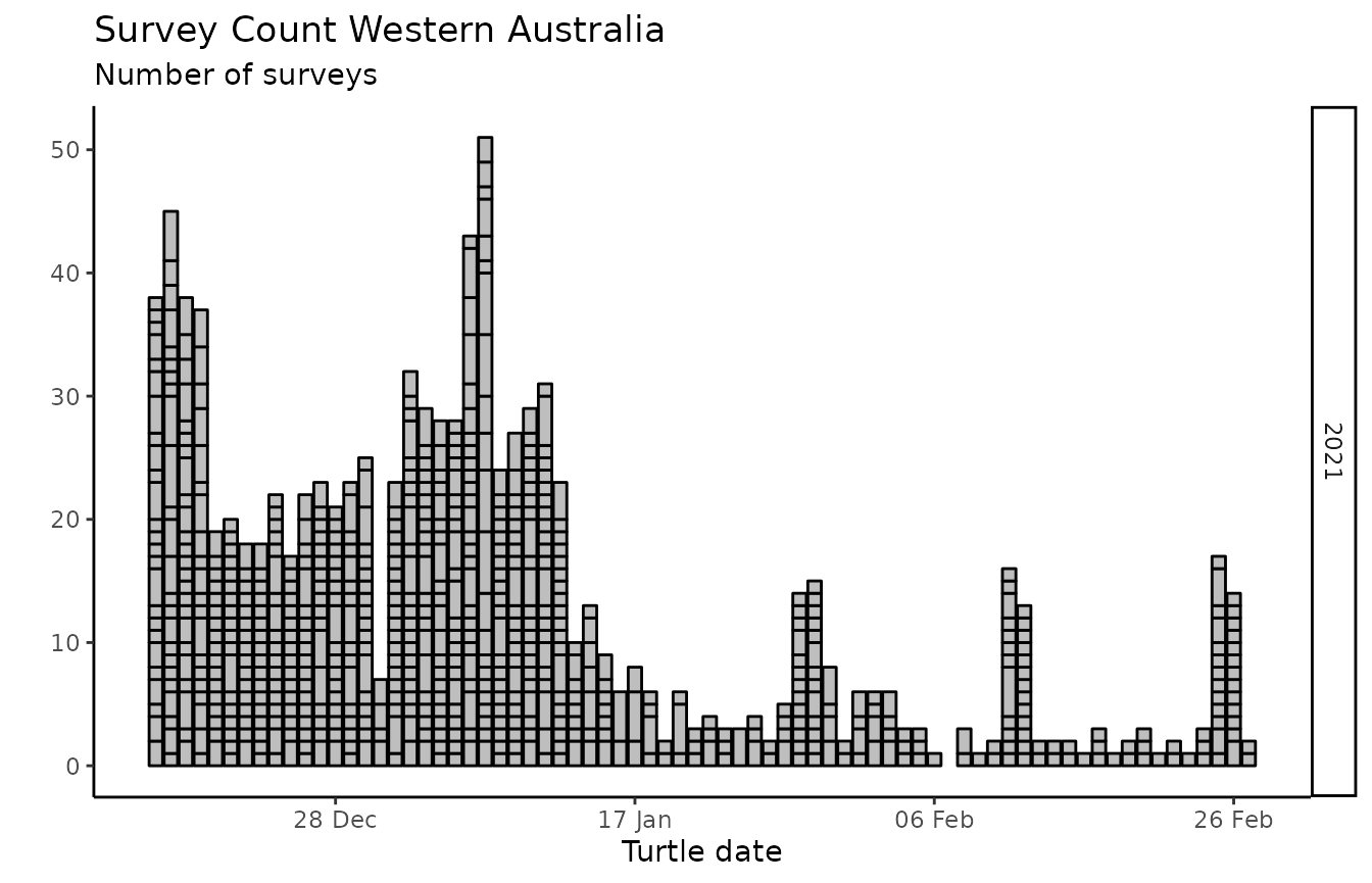

wastd_data$surveys %>% survey_hours_per_site_name_and_date() %>% rt()

wastd_data$surveys %>% survey_hours_per_person() %>% rt()

wastd_data$surveys %>% list_survey_count()

wastd_data$surveys %>% plot_survey_count(placename = pl, prefix = pr, export = FALSE)

wastd_data$surveys %>% list_survey_effort()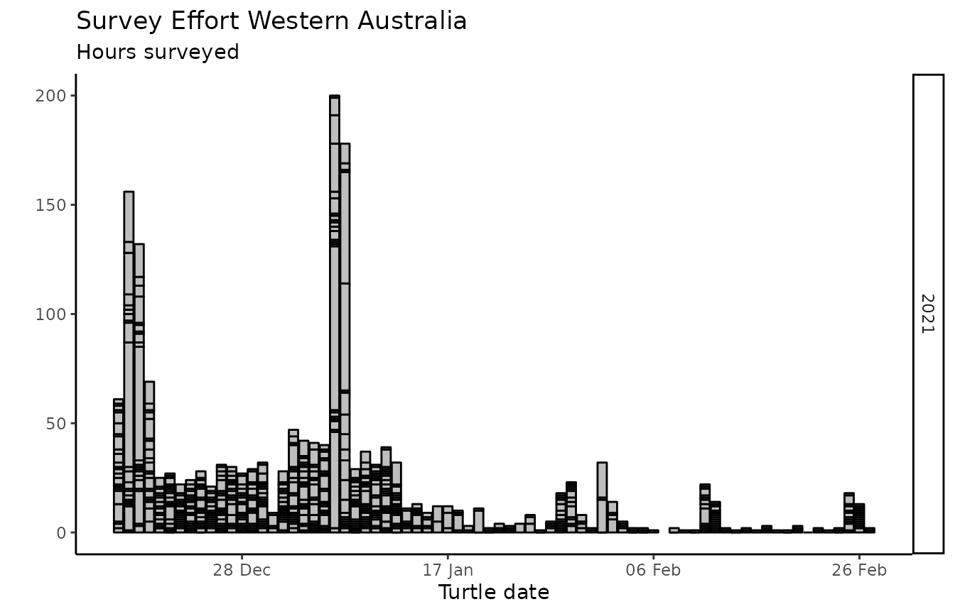

wastd_data$surveys %>% plot_survey_effort(placename = pl, prefix = pr, export = FALSE)

wastd_data$surveys %>% survey_hours_heatmap(placename = pl, prefix = pr, export = FALSE)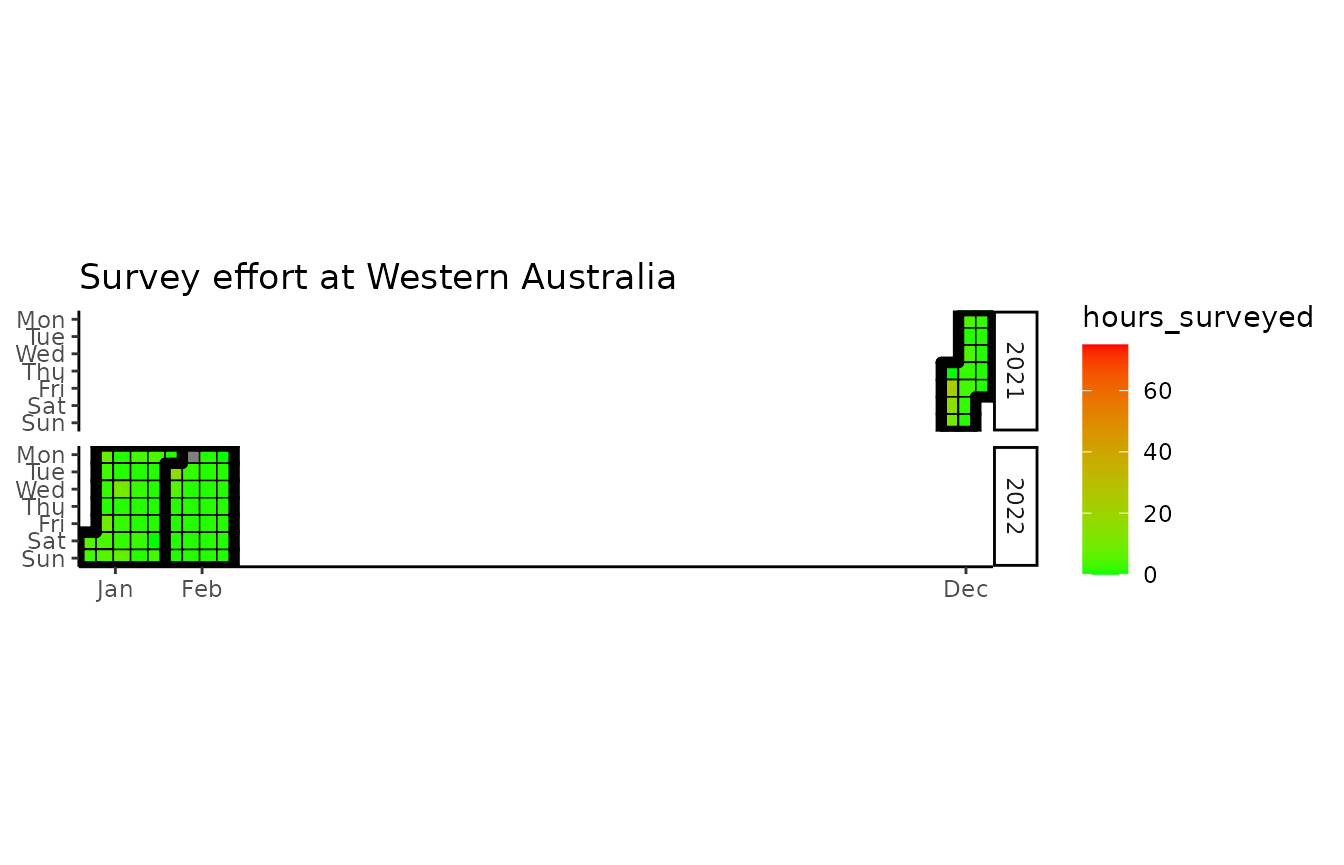

wastd_data$surveys %>% survey_count_heatmap(placename = pl, prefix = pr, export = FALSE)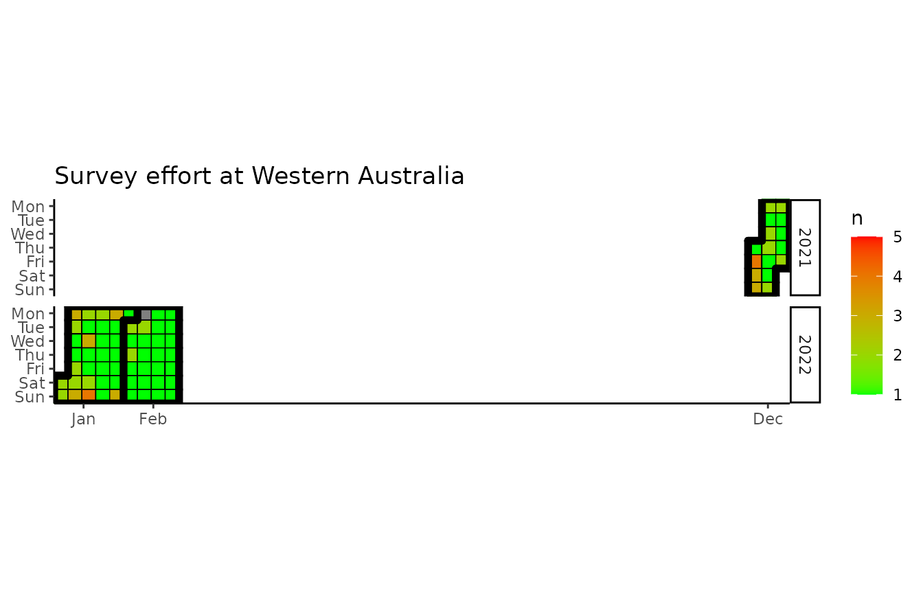

wastd_data$surveys %>%
  survey_season_stats() %>%
  rt()

wastd_data$surveys %>% survey_season_site_stats() %>% rt()

wastd_data$surveys %>% survey_show_detail() %>% rt()

QA

QA products are part of the ETL pipeline in R package etlTurtleNesting.

Currently, there are QA reports for user mapping as well as sites and surveys.

Duplicate Surveys

Sites are expected to be surveyed not more than once daily with the exception of turtle tagging, where a morning survey and night tagging can happen legitimately on the same calendar date.

QA operators will want to open each link from this list of potential duplicate surveys, inspect their details, then decide on whether to make one the main survey and close others as duplicates with the “make production” button.

wastd_data$surveys %>%
  wastdr::duplicate_surveys() %>%
  rt()